Functional Programming

Functionals, Function Factories, and Function Operators

Assignment. Practice using functionals, function factories, and function operators to improve your programming skillset.

Functionals: Run Multiple Regressions. Use a functional to fit a separate regression of mpg on each predictor. Extract the coefficient, p-value, and R² from each model. Combine the results into a data frame showing one row per predictor.

predictors <- c("disp", "hp", "wt", "qsec")

models <- purrr::map(predictors, \(x) {
  lm(reformulate(x, response = "mpg"), data = mtcars)
})
models

[[1]]

Call:
lm(formula = reformulate(x, response = "mpg"), data = mtcars)

Coefficients:
(Intercept)         disp  
   29.59985     -0.04122  


[[2]]

Call:
lm(formula = reformulate(x, response = "mpg"), data = mtcars)

Coefficients:
(Intercept)           hp  
   30.09886     -0.06823  


[[3]]

Call:
lm(formula = reformulate(x, response = "mpg"), data = mtcars)

Coefficients:
(Intercept)           wt  
     37.285       -5.344  


[[4]]

Call:
lm(formula = reformulate(x, response = "mpg"), data = mtcars)

Coefficients:
(Intercept)         qsec  
     -5.114        1.412  

results <- purrr::map_dfr(models, \(model) {
  broom::tidy(model) |>
    dplyr::filter(term != "(Intercept)") |>
    dplyr::select(term, estimate, p.value) |>
    dplyr::mutate(r_squared = broom::glance(model)$r.squared)
})
results

# A tibble: 4 × 4
  term  estimate  p.value r_squared
  <chr>    <dbl>    <dbl>     <dbl>
1 disp   -0.0412 9.38e-10     0.718
2 hp     -0.0682 1.79e- 7     0.602
3 wt     -5.34   1.29e-10     0.753
4 qsec    1.41   1.71e- 2     0.175

Function Factories: Create a Model Factory. Create a function called make_modeler that takes a dataset and an outcome variable and returns a function that fits a linear model using a predictor supplied later. Use it to fit models predicting mpg and modify the returned function so it returns a tidy summary of the model rather than the entire model object.

make_modeler <- function(data, outcome) {
  function(predictor) {
    model <- lm(reformulate(predictor, response = outcome), data = data)
    tidymodel <- broom::tidy(model) |>
      dplyr::filter(term != "(Intercept)")
    return(tidymodel)
  }
}

model_mpg <- make_modeler(mtcars, "mpg")

purrr::map_dfr(c("wt", "hp", "disp", "qsec"), model_mpg)

# A tibble: 4 × 5
  term  estimate std.error statistic  p.value
  <chr>    <dbl>     <dbl>     <dbl>    <dbl>
1 wt     -5.34     0.559       -9.56 1.29e-10
2 hp     -0.0682   0.0101      -6.74 1.79e- 7
3 disp   -0.0412   0.00471     -8.75 9.38e-10
4 qsec    1.41     0.559        2.53 1.71e- 2

Julianne making more practice examples

library(palmerpenguins)

penguin_modeler <- function(data, outcome) {
  function(predictor) {
    model <- lm(
      reformulate(predictor, response = outcome),
      data = data
    )
    broom::tidy(model)
  }
}

model_bill <- penguin_modeler(penguins, "body_mass_g")
model_bill

function (predictor) 
{
    model <- lm(reformulate(predictor, response = outcome), data = data)
    broom::tidy(model)
}
<environment: 0x558f5c83bad0>

model_bill("bill_length_mm")

# A tibble: 2 × 5
  term           estimate std.error statistic  p.value
  <chr>             <dbl>     <dbl>     <dbl>    <dbl>
1 (Intercept)       362.     283.        1.28 2.02e- 1
2 bill_length_mm     87.4      6.40     13.7  3.81e-34

predictors_penguin <- c(
  "bill_length_mm",
  "bill_depth_mm",
  "flipper_length_mm"
)

purrr::map_dfr(predictors_penguin, model_bill)

# A tibble: 6 × 5
  term              estimate std.error statistic   p.value
  <chr>                <dbl>     <dbl>     <dbl>     <dbl>
1 (Intercept)          362.     283.        1.28 2.02e-  1
2 bill_length_mm        87.4      6.40     13.7  3.81e- 34
3 (Intercept)         7489.     335.       22.3  1.13e- 68
4 bill_depth_mm       -192.      19.4      -9.87 2.28e- 20
5 (Intercept)        -5781.     306.      -18.9  5.59e- 55
6 flipper_length_mm     49.7      1.52     32.7  4.37e-107

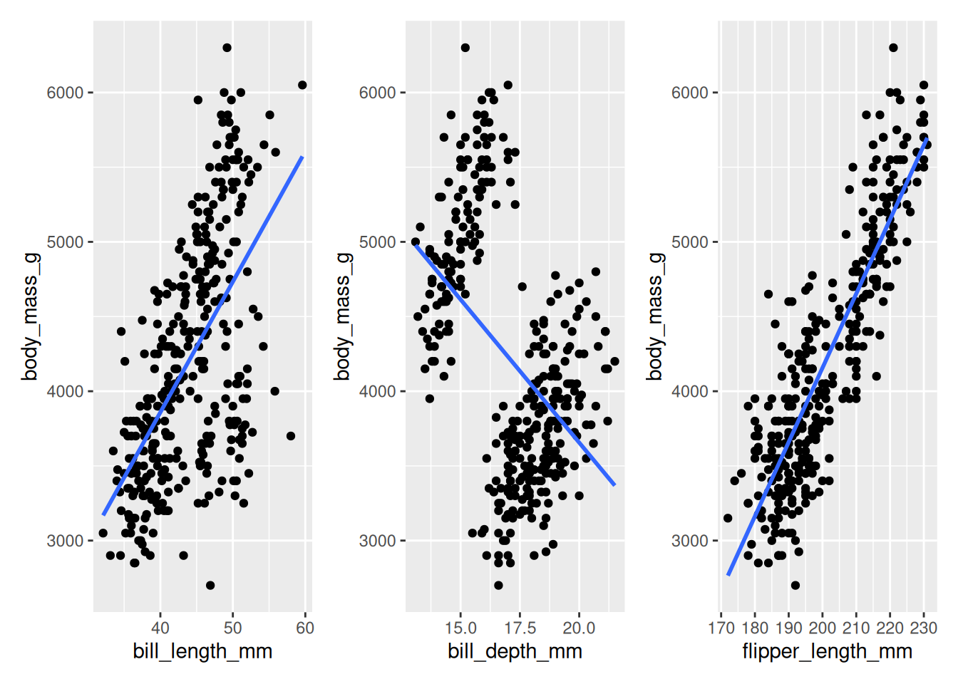
plotting practice

library(ggplot2)

make_plotter <- function(data, outcome) {
  function(predictor) {
    ggplot(
      data,
      aes(x = .data[[predictor]], y = .data[[outcome]])
    ) +
      geom_point() +
      geom_smooth(method = "lm", se = FALSE)
  }
}

penguin_body_mass_plotter <- make_plotter(
  penguins,
  "body_mass_g"
)

predictors_plot <- c(
  "bill_length_mm",
  "bill_depth_mm",
  "flipper_length_mm"
)

plots <- purrr::map(
  predictors_plot,
  penguin_body_mass_plotter
)

patchwork::wrap_plots(plots)