Object-Oriented Programming

Functionals, Function Factories, and Function Operators

Assignment. Practice functional (S3) and encapsulated (R6) object-oriented programming.

S3 Objective: Practice creating S3 classes and defining class-specific methods for generic functions. Using the mtcars dataset, fit a linear regression model predicting mpg from wt, cyl, and hp. Assign the model a custom class called rlab_lm, while retaining its existing “lm” class.

Implement the following methods:

1. print.rlab_lm() — Print a concise summary of the model that includes:

• The intercept
• The beta coefficients for each predictor
• The model’s (R²)
• The sample size Round numerical results to two decimal places by default.

2. summary.rlab_lm() — Return a data frame containing the coefficient names, estimates, (R²), and sample size.

Requirements:

• Use S3 method naming conventions.
• Use class() to assign the custom class.
• Ensure that both methods work when called through the generic functions print() and summary().
• Avoid recursive calls between your custom methods and the generic functions.

Challenge: Modify the print method to allow users to control the number of decimal places with a digits argument.

rlab_lm <- function(data, response, ...) {
  pred <- list(...)
  termlabels <- paste0(unlist(pred), collapse = " + ")
  fm <- as.formula(reformulate(termlabels, response))
  fit <- lm(fm, data = data)
  # Assign a custom S3 class
  class(fit) <- c("rlab_lm", class(fit))
  return(fit)
}

print.rlab_lm <- function(object, digits = 2, ...) {
  model_summary <- summary.lm(object)
  estimates <- round(coef(object), digits)
  intercept <- estimates["(Intercept)"]
  betas <- estimates[names(estimates) != "(Intercept)"]
  beta_labels <- paste0(names(betas), ": ", unname(betas))

  cat("Linear Regression Model\n")
  cat("-----------------------\n")
  cat("Intercept:", unname(intercept), "\n")
  cat("Coefficients:", paste(beta_labels, collapse = ", "), "\n")
  cat("R-squared:", round(model_summary$r.squared, digits), "\n")
  cat("Sample size:", nobs(object), "\n")

  invisible(object)
}

summary.rlab_lm <- function(object, digits = 2, ...) {
  estimates <- round(coef(object), digits)
  model_summary <- summary.lm(object)
  out <- as.data.frame(t(estimates))
  out$r_squared <- round(model_summary$r.squared, digits)
  out$n <- nobs(object)
  out
}

print(rlab_lm(mtcars, response = "mpg", "wt", "cyl", "hp"), digits = 3)

Linear Regression Model
-----------------------
Intercept: 38.752 
Coefficients: wt: -3.167, cyl: -0.942, hp: -0.018 
R-squared: 0.843 
Sample size: 32 

summary(rlab_lm(mtcars, response = "mpg", "wt", "cyl", "hp"), digits = 6)

  (Intercept)        wt       cyl        hp r_squared  n
1    38.75179 -3.166973 -0.941617 -0.018038   0.84315 32

R6 Objective. In this activity you’ll build a virtual deck of playing cards using R6. You’ll start with a plain vector of 52 cards, then wrap it in an R6 class so you can write deck$shuffle() and deck$draw(5) the way you’d use a real deck. By the end, you’ll know how to:

• Define a class with R6Class()
• Store data in a field and write methods that use it
• Use self to refer to the object’s own data
• Chain methods together (deck$shuffle()$draw(5))

Deck <- R6::R6Class(
  "Deck",
  public = list(
    cards = NULL,

    initialize = function() {
      suits <- c("♠", "♥", "♦", "♣")
      values <- c("A", 2:10, "J", "Q", "K")
      self$cards <- paste0(rep(values, times = 4), rep(suits, each = 13))
    },

    shuffle = function() {
      self$cards <- sample(self$cards)
      invisible(self)
    },

    draw = function(n = 1) {
      drawn <- self$cards[seq_len(n)]
      self$cards <- self$cards[-seq_len(n)]
      drawn
    },

    reset = function() {
      self$initialize()
      invisible(self)
    },

    plot = function(cards = self$cards, ...) {
      idx <- seq_along(cards) - 1
      card_df <- data.frame(
        x = idx %% 13,
        y = -(idx %/% 13),
        label = cards,
        suit = substr(cards, nchar(cards), nchar(cards))
      )

      ggplot2::ggplot(card_df, ggplot2::aes(x, y)) +
        ggplot2::geom_tile(
          width = 0.9,
          height = 0.95,
          fill = "white",
          color = "grey40"
        ) +
        ggplot2::geom_text(
          ggplot2::aes(label = label, color = suit),
          size = 6
        ) +
        ggplot2::scale_color_manual(
          values = c("♠" = "black", "♥" = "red3", "♦" = "red3", "♣" = "black")
        ) +
        ggplot2::coord_fixed() +
        ggplot2::theme_void() +
        ggplot2::theme(legend.position = "none")
    }
  )
)

# Create a new deck
deck <- Deck$new()

# Draw 5 cards before the deck is shuffled and plot the output
hand <- deck$draw(5)

deck$plot(hand)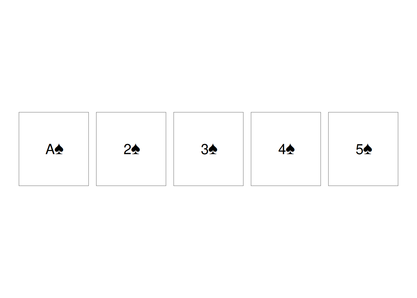

# Draw 5 cards after the deck is shuffled and plot the output
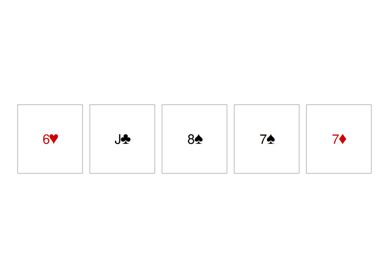
shuffled_hand <- deck$shuffle()$draw(5)

deck$plot(shuffled_hand)